Functionalities

eTraGo is based on the open source tool PyPSA and uses its definitions and units [PyPSA].

Data Model

The model covers the coupling of electricity grid models on different voltage levels with gas grid models (depending on the scenario considered) and captures sectoral demands and flexibilities from electricity, mobility, heat, and gas systems, including further electrical flexibilities such as demand-side management and dynamic line rating. It is characterised by a high spatial resolution within Germany, while other countries are considered in an aggregated form. Several future scenarios have been developed, each covering one year in hourly resolution and differing in terms of generation, demand and availability of some technologies. The data model is generated using the tool eGon-data. More details on the model can be found in the documentation of eGon-data or the following publications: [eGon_report] and [Buettner2024]. The graphs below give some impressions [eGon_report]:

eTraGo fetches the input data from the Open Energy Platform when the db argument is set to ‘oep’. Alternatively, different scenarios of the data models are available through zenodo. The data needs to be downloaded and locally stored as a PostgreSQL database to be accessable for eTraGo. More explanations can be found in this zenodo upload. The following scenarios are available:

Scenario name	Description	Status	Accessible at
status2019	Represents the system status in 2019	computable	Zenodo
eGon2035	Based on scenario C2035 from the Network Development Plan ([NEP]), version 2021	computable	Open Energy Platform or Zenodo
eGon2035_lowflex	Variant of eGon2035 with lower penetration of flexibilities	computable	Open Energy Platform or Zenodo
eGon100RE	Characterised by 100% renewable generation	under development	–

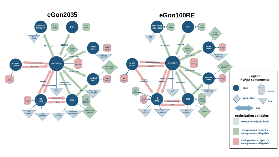
You can see the modeling concepts of the scenarios in the figure below. The components marked green have exogenous capacity and endogenous dispatch whereas the components marked in red are optimized endogenously in capacity and dispatch.

In addition, you can choose extension scenarios which will be added to the existing network container (e.g. to add new planned lines). In case new components replace existing ones, these are dropped from the network. Data of the extension scenarios is located in specific extension tables (e.g. grid.egon_etrago_extension_line). The following extension scenarios are available:

Scenario name	Description	Status	Accessible at
nep2021_confirmed	Includes all planed new lines confirmed by the Bundesnetzagentur included in the NEP version 2021	computable	Zenodo
nep2021_c2035	Includes all new lines planned by the Netzentwicklungsplan 2021 in scenario 2035 C	computable	Zenodo

Consideration of Simplified Distribution Grids

To improve flexibility dispatching in the underlying distribution grids, they can be considered in a simplified way within eTraGo. When this option is selected, distribution grid buses are added to each HV/MV substation in the transmission grid. The transmission and distribution grid buses are connected via a link component. This component is parametrized in terms of capacity and expansion costs, which model the simplified exchange between the two grid levels. These parameters are derived from simulations within eDisGo via eGo. If you only intend to run eTraGo, you can import predefined data from a CSV file. Generation, load, and storage unit components are connected to their respective grid levels using original, non-aggregated data from the database. As a result, the modeling concept is adjusted as follows (illustrated here using the eGon2035 scenario):

Scenario Variation

Several features were developed to enhance the functionality of eTraGo and allow for adaptions within the scenarios introduced above.

• In ‚extendable‘ you can adapt the type of components you want to be optimized in capacity and set upper limits for grid expansion inside Germany and of lines to foreign countries.

• With ‘foreign_lines‘ you can adapt the foreign lines to be modeled as DC-links (e.g. to avoid loop flows).

• ‘branch_capacity_factor’ adds a factor to adapt all line capacities in order to consider (n-1) security. Because the average number of HV systems is much smaller than the one of eHV lines, you can choose factors for ‘HV’ and ‘eHV’ separately.

• The ‚extra_functionality‘-argument allows to consider extra constraints like limits for energy imort and export or minimal renewable shares in generation.

• The ‘load_shedding’-argument is used for debugging complex grids in order to avoid infeasibilities. It introduces a very expensive generator at each bus to meet the demand. When optimizing storage units and grid expansion without limiting constraints, the need for load shedding should not be existent.

Complexity Reduction

The data model is characterised by a high spatial (about 8,000 electrical and 600 gas nodes) and temporal resolution (8,760 timesteps). To reduce the complexity of the resulting optimization problem, several methods can be applied. Those methods are implemented within the package etrago.cluster.

Reduction in Spatial Dimension:

The ehv clustering maps all electrical nodes with a voltage level below the extra-high voltage level to their nearest neighboring node in the extra-high voltage level with the Dijkstra’s algorithm (110 kV —> 220 kV / 380 kV).

The k-means Clustering reduces the electrical or gas network to an adjustable number of nodes by considering the geographical position of the respective nodes. This method has been implemented within PyPSA by [Hoersch].

The k-medoids Dijkstra Clustering aggregates nodes considering the network topology. First, a k-medoids Clustering is used dividing the original nodes of the network into groups by their geographical positions while identifiying the geographical medoid nodes per cluster. Afterwards, the original nodes in the original network are assigned to the former identified medoids considering the original network’s topology applying a Dijkstra’s algorithm considering the line lengths. Afterall, the original nodes are represented by one aggregated node per cluster at the position of the former identified medoid node.

The procedures of the two methods are depicted in the following figure [Esterl2024]:

Additionally, there is the option to perform a clustering with a focus on a defined region, in which the spatial distribution of clustered buses is intentionally weighted toward the corresponding region. This allows a higher spatial resolution within and around the region of interest, while areas farther away are represented with fewer buses.

In general, the clustering of the sector-coupled system is divided into two steps: First, the electrical and gas grid are clustered independently using one of the methods described above. Afterwards, nodes of the other sectors (hydrogen, heat, e-mobility and DSM nodes) are mapped according to their connection to electricity or gas buses and aggregated to one node per carrier.

Reduction in Temporal Dimension:

The method Skip Snapshots implies a downsampling to every nth time step. The considered snapshots are weighted respectively to account for the analysis of one whole year.

By using the method called Segmentation, a hierarchical clustering of consecutive timesteps to segments with variable lengths is applied [Pineda].

The Snapshot Clustering on Typical Periods implies a hierarchical clustering of time periods with a predefined length (e.g. days or weeks) to typical periods. Those typical periods are weighted according to the number of periods in their cluster. This method optionally includes the linkage of the typical periods in a second time layer to account for the intertemporal dependencies following [Kotzur].

Calculation with PyPSA

All optimization methods within eTraGo base on the Linear Optimal Power Flow (LOPF) implemented in PyPSA. The objective is the minimization of system costs, considering marginal costs of energy generation and investments in grid infrastructure, storage units and different flexibility options. The different options are specific for each scenario. You find the implementation within the package etrago.execute.

Currently, two different optimization approaches are implemented considering different configurations of energy markets and optimization variables. The different options are described in the following sections.

Integrated Optimization with Nodal Pricing

The objective is to minimize marginal costs of energy generation and investments in grid infrastructure, storage units and different flexibility options in one optimization problem. Various constrains are added to model the physical and electrical behavior. The following objective function is applied:

This implies a nodal pricing approach with optimal dispatch and redispatch. Redispatch and curtailment of renewable energy are possible without incurring additional redispatch costs. Investments and expanded capacities of grid infrastructure, storage units, and various flexibility options are key outcomes. It should be noted that expansion is applied continuously. The expanded capacities do not always reflect existing technical constraints, which allows the optimization problem to remain linear and feasible for the complex model described.

The integrated optimization produces highly cost-effective results, but it does not fully reflect the actual German energy market. A more detailed description of this modeling approach, as well as selected results, can be found in various studies and papers, e.g., [Mueller2019] and [Buettner2024].

Consecutive Market and Grid Optimization

This methodology aims to represent an energy market close to the current market design by separating the market model from the grid model. The optimization method consists of three consecutive steps.

First, seasonal storage behavior and market-based expansions of flexibility options are identified through a simplified yet annual calculation. The second step generates a realistic dispatch for each power plant and hour, taking into account non-linear Unit Commitment constraints and a short-term, rolling planning horizon. In both steps, the spatial resolution is defined as one node per current bidding zone.

In the final optimization step, the grid topology (potentially in a reduced spatial resolution as described in [Buettner2024]) is considered, allowing for optimization of grid expansion. The market-based dispatch is determined by the previous step; redispatch and curtailment are possible, but they result in additional system costs.

A brief overview of the different optimization steps, their key characteristics and results is shown in the following figure. A detailed description of the methodology is given in [Buettner20242], which also presents and analyses results.

Grid and Storage / Store Expansion

The grid expansion is realized by extending the capacities of existing lines and substations. These capacities are considered as part of the optimization problem whereby the possible extension is unlimited. With respect to the different voltage levels and lengths, MVA-specific costs are considered in the optimization.

As shown in the figure above, several options to store energy are part of the modeling concept. Extendable batteries (modeled as storage units) are assigned to every node in the electrical grid. A minimum installed capacity is being considered to account for home batteries ([NEP]). The expansion and operation is part of the optimization. Furthermore, two types of hydrogen stores (modeled as stores) are available. Overground stores are optimized in operation and dispatch without limitations whereas underground stores depicting saltcaverns are limited by geographical conditions ([BGR]). Additionally, heat stores part of the optimization in terms of power and energy without upper limits.

Non-Linear Power Flow

With the argument ‘pf_post_lopf’, after the LOPF a non-linear power flow simulation can be conducted.

Solver Options

To customize computation settings, ‘solver_options’ and ‘generator_noise’ should be adapted. The latter adds a reproducible small random noise to the marginal costs of each generator in order to prevent an optima plateau. The specific solver options depend on the applied solver (e.g. Gurobi, CPLEX or GLPK).

Insights on Solver Settings with Gurobi

• threads: number of threads to apply to parallel algorithms (concurrent or barrier)

  • default: 0 (uses all cores in the machine)

  • reduce if parallel calculations or tight memory

• method: algorithm used to solve optimization of lopf

  • default (-1, concurrent): chooses between simplex or barrier method due to matrix range

  • 1 (simplex): slower but less sensitive for numerical issues

  • 2 (barrier): fastest method but sensitive for numerical issues

• crossover (barrier only): determines the crossover strategy used to transform the interior solution produced by barrier into a basic solution

  • default: -1 (chooses strategy automatically)

  • preferred: 0 (disables crossover, solves fastest but may need ‘NumericFocus’ and ‘BarHomogenus’ to avoid numerical issues)

• BarConvTol (barrier only): the barrier solver terminates when the relative difference between the primal and dual objective values is less than the specified tolerance

  • default: 1e-8

  • preferred: 1e-5 (little less accurate, but solves faster)

• FeasibilityTol: tolerance of all constraints

  • default: 1e-6

  • preferred: 1e-5 (less accurate, but reduces number of iterations)

• logFile: destination and name of gurobi log file

  • default: None

  • preferred: ‘gurobi_eTraGo.log’

• BarHomogeneous: (barrier only): determines whether to use the homogeneous barrier algorithm

  • default: -1 (homogeneous barrier algorithm turned off, faster but sensitive for numerical issues)

  • preferred: 1 (homogeneous barrier algorithm turned on, bit slower but less sensitive for numerical issues, often used when crossover turned off)

• NumericFocus: controls the degree to which the code attempts to detect and manage numerical issues

  • default: 0 (automatic choice with a slight preference for speed)

  • 1 - 3 (shift the focus towards being slower but less sensitive for numerical issues)

Disaggregation

By applying a 2-level-approach, a temporal disaggregation can be conducted. This means optimizing dispatch using the fullcomplex time series in the second step after having optimized grid and storage expansion using the complexity-reduced time series in the first step. More information can be found in the master thesis by [Esterl2022].

Afterterwards, a spatial disaggregation can be conducted distributing power plant and storage utilisation time series, the expansion of storage facilities and the use of flexibility options over the original number of nodes. The expansion of the transmission grid is not disaggregated and remains at the reduced spatial resolution. The methodology is explained in [eGon_report].

The corresponding methods are implemented as part of the package etrago.disaggregate

Analysis

eTraGo contains various functions for evaluating the optimization results in the form of graphics, maps and tables. Functions to quantify results can be found in etrago.analyze.calc_results() and functions to plot results can be found in etrago.analyze.plot. Some examplary graphs by [Buettner2024] are presented below: